
Microsoft Excel is usually used for calculations and adding formulas. However, the software can be used as a full-fledged data entry tool by using powerful data validation features and options. In this blog post, I will explain to you how you can combine Data Validation and Dynamic Named Ranges to ensure that valid data is entered and incorrect entries are not allowed by flagging an error.
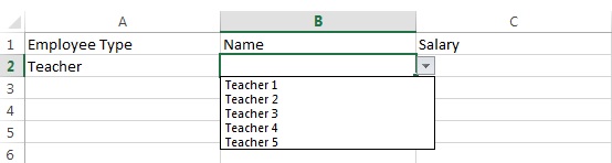
Suppose you work in a school. The school has the teaching staff, the operations staff, and the managerial staff. In an Excel Sheet, you want to enter details of each employee in three columns. Column A shows the Employee Type (Teacher, Operations, Managerial Post). Column B shows the Name of the employee. The Salary is entered in Column C.
The requirement is as follows: Column A should only allow the entry of the values Teacher, Operations, and Managerial Post (Employee Type). Column B should be a dependent dropdown. and the values should change based on what is entered in Column A. So, for example, if Teacher is selected in Column A, Column B dropdown should show only teacher names. If Managerial Post is selected in Column A, Column B dropdown should show only manager names. Column C should allow entering only numbers in salary with no decimal places.
Let’s create an Excel File to accomplish all these objectives. I have named the Excel File data.xlsx. Follow these steps. The finalized file will look similar to the following snapshots:
- In Sheet1, Cell A1, enter Employee Type
- In Cell B1, enter Name
- In Cell C1, enter Salary
- Now create another sheet Sheet2
- In Sheet2, Cell A1, enter Employee Type
- In Sheet2 , from A2 to A4, enter A2 = Teacher, A3 = Operations, and A4 = Managerial Post
- Place the cursor in Sheet2, Cell A1, and select FORMULAS -> Define Name -> Define Name…
- In Refers to: enter the following formula:
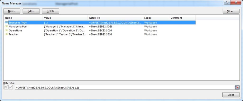
=OFFSET(Sheet2!$A$2,0,0,COUNTA(Sheet2!$A:$A)-1,1)- Click OK. You have now created a range named Employee_Type. You could have simply entered:
=Sheet2!$A$2:$A$4- but it would not have created a dynamic range. The use of the OFFSET formula has made the range dynamic. So, for example, if you enter another category in A5, it will automatically be included in the range Employee_Type.
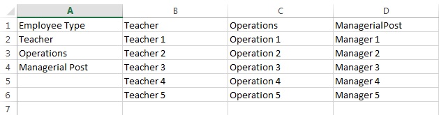
- In Sheet2, enter B1=Teacher, C1=Operations, D1=ManagerialPost. Note that there is no space in ManagerialPost because a named ranged cannot include a space. Otherwise, the names match exactly with the entries in the Employee Type list.
- Now enter five values from B2 to B6 in Sheet2 as follows: B2=Teacher 1, B3=Teacher 2, B4=Teacher 3, B5=Teacher 4, B6=Teacher 5.
- Now enter five values from C2 to C6 in Sheet2 as follows: C2=Operation 1, C3=Operation 2, C4=Operation 3, C5=Operation 4, C6=Operation 5.
- Now enter five values from D2 to D6 in Sheet2 as follows: D2=Manager 1, D3=Manager 2, D4=Manager 3, D5=Manager 4, D6=Manager 5.
- Place your cursor on Sheet2, Cell B1, and click FORMULAS -> Define Name -> Define Name…
- In Refers to: enter the following and click OK:
=Sheet2!$B$2:$B$6- Place your cursor on Sheet2, C1, and click FORMULAS -> Define Name -> Define Name…
- In Refers to: enter the following and click OK:
=Sheet2!$C$2:$C$6- Place your cursor on Sheet2, D1, and click FORMULAS -> Define Name -> Define Name…
- In Refers to: enter the following and click OK:
=Sheet2!$D$2:$D$6- Click FORMULAS -> Name Manager. It will list all the Named Ranges created by you and the output should match the following snapshot:
- Go to Sheet1
- In Sheet1, cell A2, you have to allow only valid entries for Employee Type. Therefore click DATA -> Data Validation -> Data Validation…
- In the Validation criteria, under Allow, select List
- In Source, enter the following, and click OK
=Employee_Type- Now click the dropdown in A2. You will see the valid values Teacher, Operations, Managerial Post. You can only select these values. Try entering anything else, and you will see the error message: ‘The value you entered is not valid’. If you add another value in the Employee Type List/Range in Sheet2, it will automatically appear in the dropdown.
- Now place the cursor in Sheet1, B2.
- Click DATA -> Data Validation -> Data Validation…
- In Validation criteria, under Allow, select List
- In Source, enter the following, and click OK. You will receive a message: ‘The Source currently evaluates to an error. Do you want to continue?‘ Ignore this error and click Yes
=INDIRECT(A2)- Now in Sheet1, A2, select Teacher from the dropdown. Now check the dropdown in B2. It will only show teachers from Teacher 1 to Teacher 5. Select Operations in A2. B2 will only show Operations Employees from Operation 1 to Operation 5. Select Managerial Post in A2, B2 will now show nothing. It occurred because the entry ‘Managerial Post’ has a space in between and the range ManagerialPost is without space. The Range Name should map exactly to the Employee Type Entry for the INDIRECT formula to work.
- To address this issue, a change in the formula will be needed. Place your cursor in Sheet1, B2, and click DATA -> Data Validation -> Data Validation…
- In Source, enter the following and click OK:
=INDIRECT(SUBSTITUTE(A2," ",""))- Now the data entry system is almost complete with full data validation. If you select Teacher in A2, B2 will allow selecting Teacher 1 to Teacher 5. When you select Operations in A2, B2 will allow selecting Operation 1 to Operation 5. If Managerial Post is selected in A2, B2 will allow selecting Manager 1 to Manager 5.
- Now, the only validation required is in Sheet1, Column C.
- Place the cursor in Sheet 1, C2. Select DATA -> Data Validation -> Data Validation…
- In Validation criteria, under Allow, select Whole number. Select Minimum (such as 1000) and Maximum (such as 1000000), and click OK. Now only whole numbers can be entered in the Salary column between 1000 and 1000000. Decimals and alphabets will not be allowed.
- Clear all entries in Sheet1, A2, B2, and C2.
- Select from A2 to C2.
- Click Copy.
- Select from A3 to C25.
- Select the down arrow of Paste and select Paste Special…
- Select Validation under Paste and click OK.
- You will see that the validation is now applied from A2 through C25.
- In this way, you can apply Validation to as many cells as you like.
Some Points to Consider
- There are some limitations of this interface that you should consider. For example, select Teacher in A2 and Teacher 2 in B2. Now select Operations in A2, B2 will still show Teacher 2, which is not correct. So, on the Worksheet Change Event, cell B2 should be cleared when there is a change in cell A2. If you want to implement it, save the file as data.xlsm (Macro-Enabled File).
- Open data.xlsm.
- Press Alt+F11 to enter the programming interface of Microsoft Visual Basic for Applications
- In Project Explorer, double-click Sheet 1 (Sheet 1)
- From the first dropdown, select Worksheet
- From the second dropdown, select Change
- Now enter the following code:
Private Sub Worksheet_Change(ByVal Target As Range)
Application.ScreenUpdating = False
If Target.Column = 1 Then
    Target.Offset(0, 1).ClearContents
End If
Application.ScreenUpdating = True
End Sub- Select Teacher in A2 and Teacher 2 in B2. Now select Operations in A2. Teacher 2 will be cleared out in B2 and you can only enter from Operation 1 to Operation 5.
- I have implemented a dynamic range for the Master List/Range Employee_Type. Therefore, you can add more values in Employee Type in Sheet2 and it will automatically be shown in the dropdown in Sheet1 because the OFFSET function has been used to create a dynamic range. However, for the dependent ranges Teacher, Operations, and ManagerialPost, I have used simple ranges such as =Sheet2!$B$2:$B$6, =Sheet2!$C$2:$C$6, and =Sheet2!$D$2:$D$6. It is because you can’t use INDIRECT with dynamic range names. INDIRECT converts a STRING to a RANGE. In the case of a dynamic name, the string is =OFFSET(……., which cannot be converted to a range. Indirect is looking for something like =$A$1:$A$10.
- If you want to make the dependent lists dynamic too, you can create the range addresses in a cell and reference that with INDIRECT. Suppose Teacher Range is to be made dynamic. Currently, Teacher Refers to =Sheet2!$B$2:$B$6. In Sheet2, cell F1, enter the following:
= "'Sheet2'!$B$2:$B$" & COUNTA(B:B)- Select FORMULAS -> Name Manager
- Select the range Teacher and enter the following in Refers to: and click Close
=Sheet2!$F$1- Now select Sheet1 and place the cursor in cell B2.
- Select DATA -> Data Validation -> Data Validation…
- Enter the following in Source and click OK
=INDIRECT(INDIRECT(SUBSTITUTE(A2," ","")))- Please note that if you follow this approach, then you will need to make all dependent ranges dynamic by creating the range addresses in a cell. It is because the Source formula has changed from INDIRECT(A2) to INDIRECT(INDIRECT(A2)).
- In Sheet2, enter a new entry Teacher 6 in the Teacher column.
- In Sheet1, select Teacher in Employee Type. Now click the dropdown of Column B. You will see that Teacher 6 is automatically added to the dropdown list because the Teacher range is now also dynamic.
30 thoughts on “How to Create Dynamic Named Range in Excel for Data Validation and Dependent Dropdown Lists”